Tech Lessons Learned Implementing Early Intervention Systems in Charlotte and Nashville
This is the second in our three-part series “Lessons Learned Deploying Early Intervention Systems.” The first part (you can find it here) discussed the importance of data science deployments.
For the past two years, we have worked with multiple police departments to build and deploy the first data-driven Early Intervention System (EIS) for police officers. Our EIS identifies officers at high risk of having an adverse incident so the department can prevent those incidents with training, counseling, or other support. (Read our peer-reviewed articles about the project here, here, and here and our blog posts here, here, here, here, and here.) Metropolitan Nashville (MNPD) started using our EIS last fall, and Charlotte-Mecklenburg (CMPD) became the first to fully deploy it in November.
Surprisingly little has been written about deploying machine learning models, given all the talk about how machine learning is changing the world. We’ve certainly run into challenges deploying our own work that no one has discussed, as far as we know. This blog post discusses some of the statistical and computational issues we’ve encountered so others can learn from our choices, both good and bad.
Output storage: For almost all projects, DSaPP stores model information and output in the same database format. One table stores information about what we call “model groups.” A model group is a unique combination of model characteristics, such as the algorithm, hyperparameters, random seed, and features. Another table stores information about “models,” each of which is a model group fit on training data. We store all the predictions (each trained model applied to out-of-sample data) in a table and standard evaluations (e.g. accuracy, precision, recall, ROC AUC, brier score, how long it takes to train) in another. The last two tables store feature importances for the model and for each prediction. Using the database to store output makes querying and analyzing results fast and easy. Thanks to thoughtful table design and indexing, we can query billions of predictions and statistics in seconds.
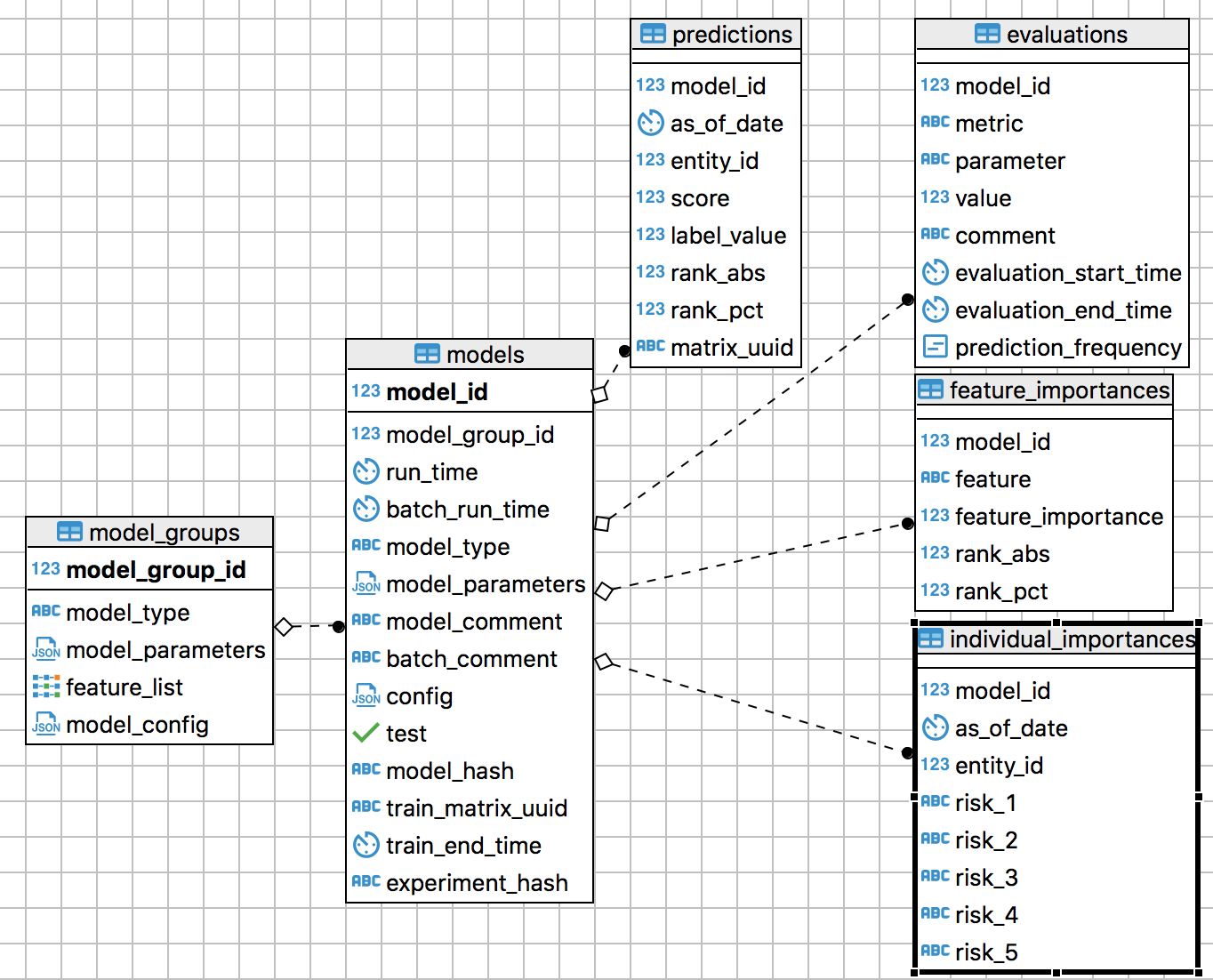 Results schema for storing model configurations and outputs
To allow future testing and development without impacting the live EIS, we created a separate “production” schema. We added new database tables for storing models, predictions, and feature importances for the models we decide to use, as well as a new “time_delta” table that stores each officer’s rank change over the past day, week, month, quarter, and year and a “review_audit” table that stores supervisor feedback for officer predictions. This schema is linked to the testing and evaluation environment by the model_group to ensure only models used in the production environment have been thoroughly tested against past data and to prevent accidental changes to the hyperparameters.
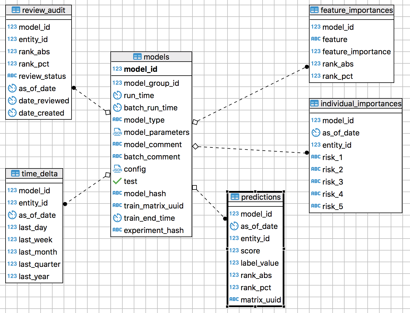
Production schema for department use
Using a standard format to store model outputs has an additional benefit: we built Tyra, a webapp that plots results for our projects. Tyra makes it easy for us and our partners to look at model performance without having to write database queries or read numbers from a table. Tyra includes precision at k over time; precision, recall, and ROC curves; feature distributions for officers with and without adverse incidents; and more. You can read more and download the code from Github: https://github.com/dssg/tyra.
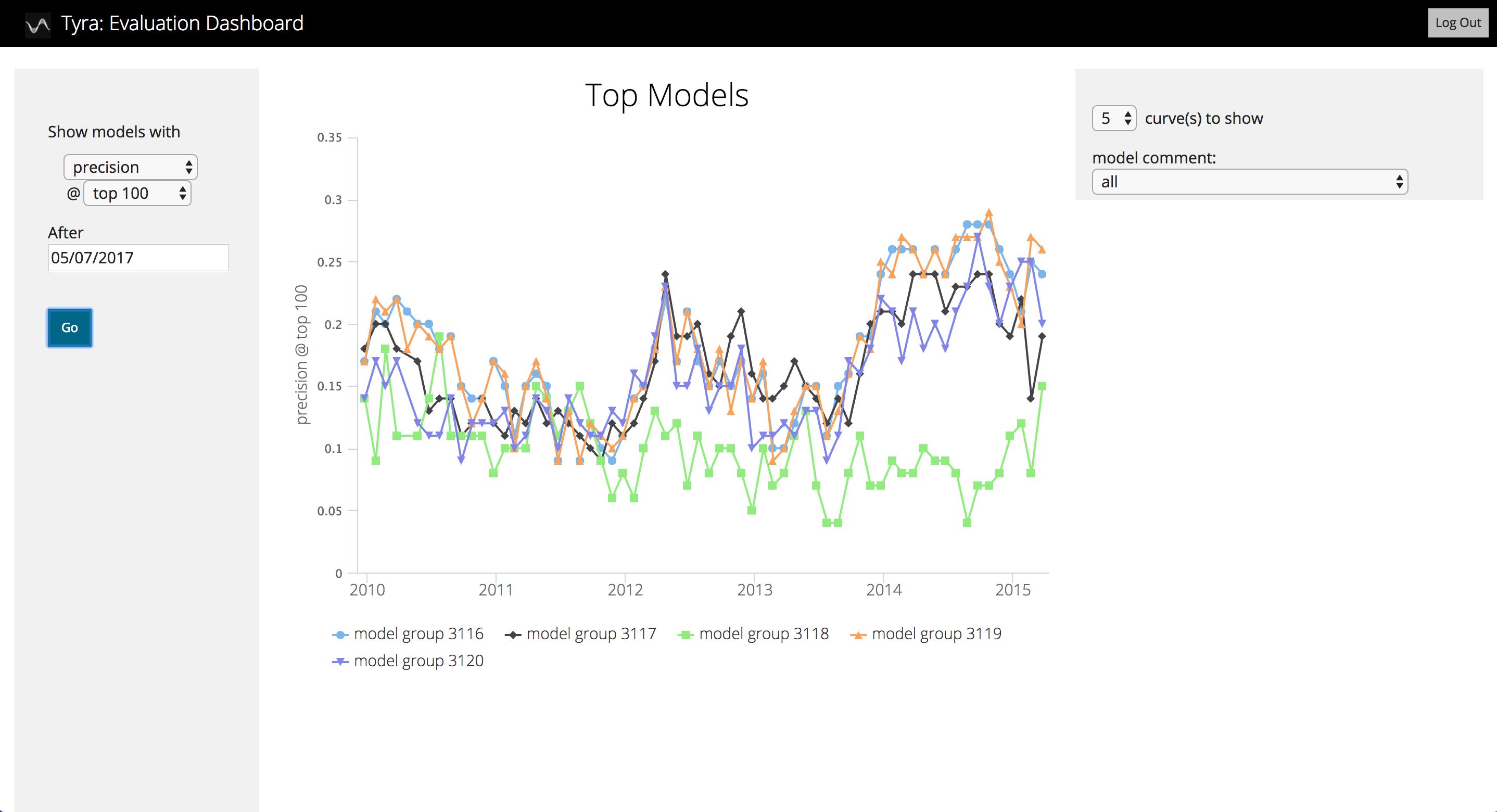
An example page from Tyra
Accuracy: Choosing a model based on its precision in one time period is asking for trouble. A model may get lucky and generate accurate predictions for that single time period but not others (including in the future). To avoid this, we want a model that generates high precision in the top 100 over time. We built checks to flag unusual changes so someone can confirm the model is still performing as expected.
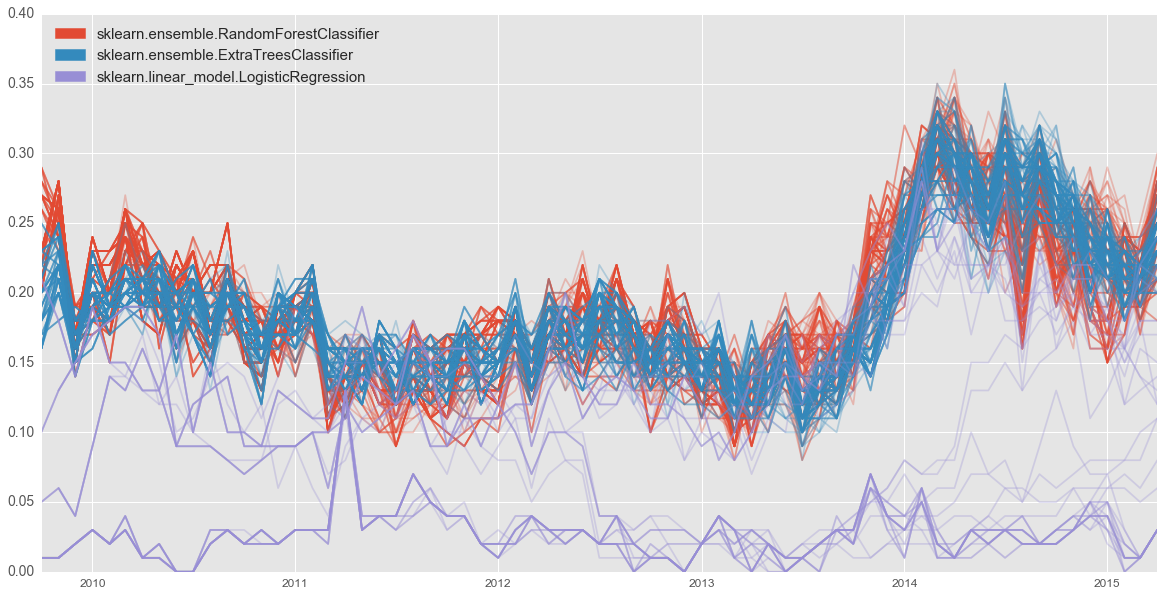
Extra trees and random forest tend to have the highest precision in the top 100. Logistic regression is the most accurate for a couple time periods. If we were to select models based on that one time period, we would choose poorly.
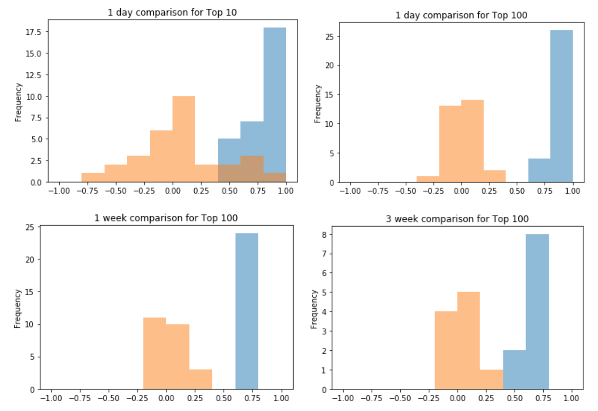
Effective interventions will reduce the value of these statistics. If the interventions are perfectly effective, the EIS will appear to have 0% precision, even if it’s 100% accurate, as the identified officers will receive interventions that prevent the adverse incident from occurring. Prediction frequency: We have published three articles on the data-driven EIS (here, here, and here). Those articles describe results for predictions made annually (e.g. every January 1st), but in practice departments will make predictions more frequently. Charlotte chose to do daily predictions, which gives them the opportunity to intervene quickly but also requires more diligence and work. Nashville chose to start with every couple months as the department learns to use an EIS. Prediction frequency affects how the EIS throws flags and how it presents flags to supervisors. An EIS that only flags officers on January 1st can simply flag the officers with the highest risk, but an EIS that generates daily predictions could flag the same officer for the same risk again and again. In Charlotte, we modified the code to stop flagging officers who have already received an EIS review or intervention. Retraining frequency: If predictive patterns hold over time, we can train a model and use it forever without loss of accuracy.[2] That’s rarely true—in an extreme example, no one would expect a model built on 19th century policing would perform as well now as it did then—so we need to retrain the model from time to time. We tested how often we need to retrain without loss of accuracy, so we know how often, at a minimum, we need to retrain. Timestamp your rows: Database administrators often overwrite data because they don’t realize how useful it might be for the EIS. Keep the old and new data by using timestamps. That way, we can recreate what was known at any given time and future updates will go faster (“only copy updated data”). Monitoring: Monitoring of any EIS is critical for success but rarely happens. Few departments can tell you how many officers their EIS flags, let alone how accurate those flags are over time. We built several automated checks to notify the department when the EIS may stop being reliable: While the list should not vary much if run twice on the same day, it should also not vary much when run the next day. If we were to generate a list of 100 officers on January 1st and a completely different list of 100 officers on January 2nd, the department would (rightly) lose confidence in the results. We should also see the top 100 officers change, as officers join and leave the department and face new circumstances. To address this, we’re checking whether Jaccard similarity (top 100) or rank-order correlation changes too little or too much.[5] We can then check whether a problem exists. Example rank-order correlations and Jaccard similarities for the EIS list. Unsurprisingly, longer lists tend to be more stable and the lists change more with time. Fixing data errors: As we’ve moved toward deployment, we’ve discovered errors in how we handled the data. Interestingly, most of those errors mean our EIS works better than expected when deployed. For example, we were selecting models using all the active officers in CMPD’s system, but it turns out many of the officers should not have been considered for evaluation. Neighboring departments use CMPD’s computer system to handle officer activities like arrests but not for internal affairs, which means those officers could never have adverse incidents and their departments could never provide interventions. We found that issue by confirming specific numbers with CMPD (e.g. number of officers on a given day, number of officers with an adverse incident, and number of adverse incidents). We plan to release another blog post soon that discusses human aspects of machine learning deployment. Please check back regularly to catch the latest. Footnotes:
We’ve had different input issues in Charlotte and Nashville. CMPD is running everything on their side, so we’re not directly involved. But we have a static data dump, and comparing the number of tables, rows, officers, adverse incidents, and other types of events for each officer has helped identify input issues. In addition, CMPD is copying updates from their results schema to our server so we can monitor their EIS.
MNPD gave us access to an analytics and postgres server, which makes it easier to help them change and implement the EIS. They created views in their production database that our postgres server accesses with a foreign data wrapper, which offers adequate performance (EISs aren’t mission critical the way, say, dispatch systems are) while enabling them to do most of their work in the database they know well.
 The proportion of officers who appear on two lists generated by the same random forest model. As we increase the number of trees in the random forest, the list of the top 100 becomes more stable.